How to Use XLOOKUP with Multiple Criteria in Excel Tables

When using the XLOOKUP function in Excel, tables are usually merged by a single column, for example the ID. But in real data there are often situations where the ID alone is not enough.

In such cases XLOOKUP may return the wrong result even though the formula is written correctly. The problem lies not in the formula, but in the chosen lookup logic.

If you are just learning the basic XLOOKUP logic, you can first read the article:how to merge Excel tables by ID using XLOOKUP.

1. Why a single lookup criterion is not enough

Imagine you have a table where the same ID repeats several times, but with different dates, cities, products or values.

For example:

• the same customer may have several orders
• the same ID may be linked to different cities
• the same product may have different prices on different days
• the same employee may be linked to several transactions

If XLOOKUP searches only by ID, it will return the first value found, which is not necessarily the one you need.

In that case you need not one, but several criteria. This lets you identify the row you actually want more precisely.

For more on why it is worth checking XLOOKUP results, see the article:how to check whether XLOOKUP results are correct.

2. The solution: multiple criteria with XLOOKUP

One of the simplest ways is to combine several criteria into a single shared lookup value.

For example, if you have:

• ID– the first criterion
• Cityordate– the second criterion

You can combine them into a single lookup logic:

This way XLOOKUP will search not only by ID, but by the ID and the second criterion together.

This lets you precisely identify the required row and avoid the situation where XLOOKUP returns the first match found, but not the one you want.

3. Practical example: merging tables by ID and city

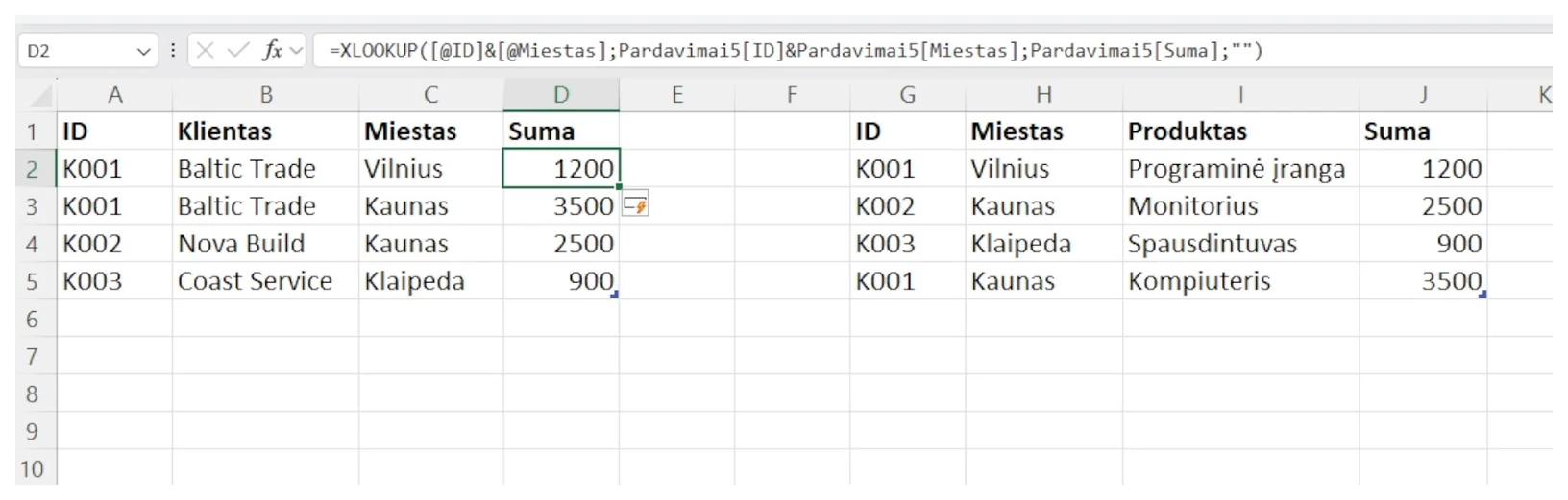
Suppose the left table contains a list of customers, and the right one contains sales information.

The problem is that the same ID can repeat more than once. For example, customer K001 may be linked to both Vilnius and Kaunas. If XLOOKUP searched only by ID, the result would not be precise enough.

In that case you can combine two criteria – ID and city.

In this formula:

• [@ID]&[@City]– combines the ID and city in the left table
• Sales[ID]&Sales[City]– combines the ID and city in the sales table
• Sales[Amount]– specifies which value to return
• “”– specifies that if the value is not found, the cell stays empty

For example:

• K001 + Vilnius → 1200
• K001 + Kaunas → 3500

This lets you merge tables accurately even when a single criterion is not enough.

Merging XLOOKUP tables by two criteria: ID and city.

4. Short video tutorial

The short tutorial below shows how to combine two criteria in an XLOOKUP formula and use them to pull a value from another table.

5. Alternative: the FILTER function

If you want more flexibility, you can use the FILTER function. It lets you return all rows that match several criteria.

For example:

This method is especially useful when:

• there may be several matches
• you need to see more than one result
• you want not just a single value, but a broader result

XLOOKUP is usually convenient when you want to return one specific result. FILTER is better suited when you need to see all rows that match the chosen logic.

6. Common mistakes

When working with multiple criteria, the following problems are common:

• spaces are left when combining criteria
• one criterion is text while the other is a number
• dates or cities are entered inconsistently in the different tables
• the criteria are combined in the wrong order

If XLOOKUP returns #N/A even though everything looks correct, the problem is very likely in the data preparation.

For more on the most common XLOOKUP problems, read the article:XLOOKUP not working? 3 most common causes and how to fix them.

Why this matters

A single-criterion lookup works for simple tables. But real data often requires more precise logic.

Using multiple criteria:

• reduces the chance of errors
• gives more precise results
• lets you work with more complex tables

This is one of the most important steps in moving from basic Excel use to more advanced work with data.

Mini course on merging Excel tables with XLOOKUP

We have prepared a short mini course that clearly shows:

• how to merge tables correctly with XLOOKUP
• when a single criterion is enough, and when you need more
• how to avoid the most common mistakes
• how to work with real data