

Most problems with XLOOKUP aren’t caused by the formula itself.
More often the problem lies in the data, its structure, or the wrong lookup logic.
So before hunting for a formula error, it’s worth checking whether the data really matches what Excel expects.
If you’re only just starting to use XLOOKUP for joining tables, you can first read the main article:how to merge Excel tables by ID using XLOOKUP.
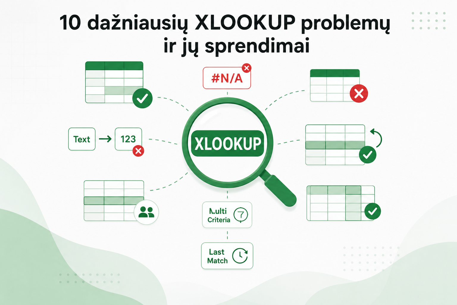
1. XLOOKUP returns #N/A
This is probably the most common problem. The #N/A error means Excel didn’t find a match in the lookup column.
If the A2 value isn’t in the ID column, you’ll get #N/A.
But the problem often isn’t that the value is missing. The most common causes are:
- hidden spaces
- different data formats
- the wrong lookup column selected
Read more about this in the article:XLOOKUP Not Working? 3 Common Causes and How to Fix Them.
2. Hidden spaces in values
Two values can look identical, but Excel treats them as different.
The second value has a trailing space. It can be hard to notice visually, but XLOOKUP won’t find such a match.
The solution is to remove the unnecessary spaces:
This is one of the most common problems when importing data from other systems.
3. Text and numbers look the same
Excel can show the same value in both tables, but in one table it may be text and in the other a number.
There’s almost no visible difference, but XLOOKUP may treat such values as different.
The solution depends on the situation. You can convert a number to text or text to a number:
4. Duplicate IDs
XLOOKUP always returns the first match it finds. This becomes a problem when the same ID appears several times in the table.
| ID | Amount |
|---|---|
| 1001 | 50 |
| 1001 | 75 |
| 1001 | 120 |
If you look up ID 1001, a normal XLOOKUP returns the first value found, even though you may have needed the last one or a specific row.
A quick check:
If the result is greater than 1, the ID is duplicated.
Read more about checking results here:how to check whether your XLOOKUP results are correct.
5. XLOOKUP returns the wrong result
This is one of the most dangerous situations: no error, no #N/A, but the result is wrong.
This usually happens because of:
- duplicate IDs
- a too-broad lookup criterion
- messy data
In this case the problem is often not in the formula, but in the lookup logic. So it’s worth checking a few rows manually and making sure XLOOKUP returns exactly the value you expect.
6. A single criterion isn’t enough
Sometimes the same ID is used several times, so the ID alone isn’t enough to identify the exact row.
In this case you build a lookup on two criteria, for example ID and date.
Read more:how to use XLOOKUP with multiple criteria in Excel tables.
7. The data is in another file
XLOOKUP can work across different Excel files.
But problems arise when:
- the file is renamed
- the file is moved
- the file becomes unavailable
Read more:how to merge Excel tables from different files with XLOOKUP.
8. You need to return multiple columns
Many users build 3–4 separate formulas, even though XLOOKUP can return several columns at once.
The result automatically spills into several columns.
Read more:how to return multiple columns at once with XLOOKUP.
9. You need the last match
By default XLOOKUP returns the first match. But sometimes you need the last one.
The parametersearch_mode = -1lets you search from the bottom of the list.
This is especially useful when looking for the last order, the latest price or the last status.
Read more:how to find the last match with XLOOKUP in Excel tables.
10. XLOOKUP or VLOOKUP: which to choose?
Although VLOOKUP is still used, XLOOKUP offers more options.
- it can look in both directions
- the formulas are clearer
- it can return several columns at once
- it can search from the bottom of the list
- errors are easier to handle
For these reasons, XLOOKUP is the more convenient choice in most cases.
Read more:XLOOKUP vs VLOOKUP: what’s the difference and which to use.
Why this matters
The more you work with Excel, the more often you deal with joining tables.
Being able to quickly diagnose XLOOKUP problems lets you:
- save time
- reduce the number of errors
- build more reliable reports
- work with data more efficiently
A mini-course on joining Excel tables with XLOOKUP
We’ve prepared a short mini-course that clearly shows:
- how to join tables with XLOOKUP
- how to avoid the most common mistakes
- how to check the results
- how to work with real data
Want to learn to join Excel tables without errors?
The mini-course shows not only how to write XLOOKUP formulas, but also how to make sure the results are correct.
🎓 View the mini-courseIf the button doesn’t work, open the course here:open the course
Power Query cheat sheet: automate your report
The key steps, the 5 common mistakes, and when automating is worth it.
- PDF · 2 pages, practical
- No spam — value only